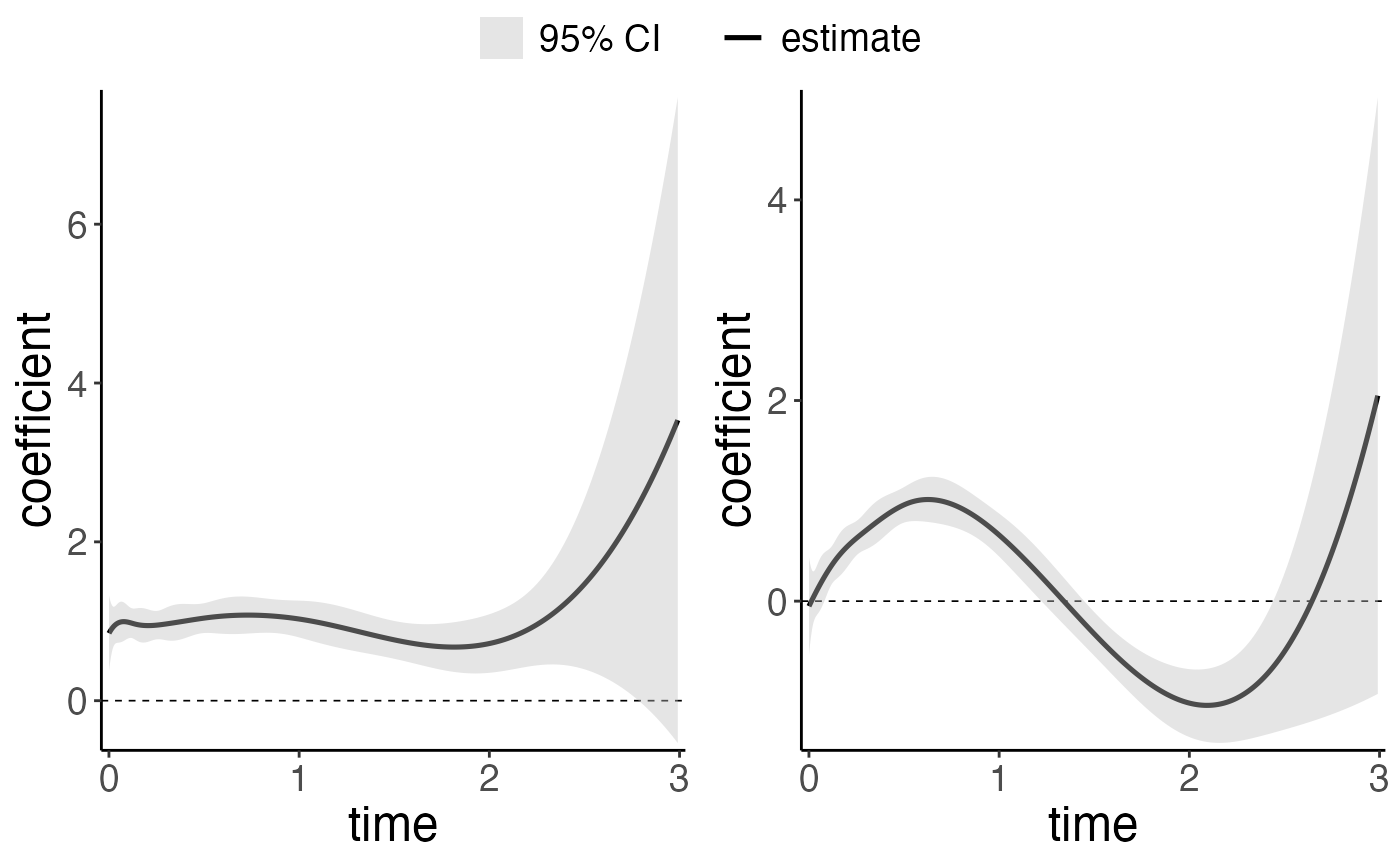
plotting results from a fitted coxtp object

This function creates a plot of the time-varying coefficients from a fitted coxtp model.

# S3 method for coxtp
plot(
  x,
  parm,
  CI = TRUE,
  level = 0.95,
  exponentiate = FALSE,
  xlab,
  ylab,
  xlim,
  ylim,
  allinone = FALSE,
  title,
  linetype,
  color,
  fill,
  time,
  ...
)

Arguments

x: model obtained from coxtp.
parm: covariate names fitted in the model to be plotted. If NULL, all covariates are plotted.
CI: if TRUE, confidence intervals are displayed. The default value is TRUE.
level: the level of confidence intervals. The default value is 0.95.
exponentiate: if TRUE, exponential scale of the fitted coefficients (hazard ratio) for each covariate is plotted. If FALSE, the fitted time-varying coefficients (log hazard ratio) are plotted.
xlab: the title for the x axis.
ylab: the title for the y axis.
xlim: the limits for the x axis.
ylim: the limits for the y axis.
allinone: if TRUE, the time-varying trajectories for different covariates are combined into a single plot. The default value is FALSE.
title: the title for the plot.
linetype: the line type for the plot.
color: the aesthetics parameter for the plot.
fill: the aesthetics parameter for the plot.
time: the time points for which the time-varying coefficients to be plotted. The default value is the unique observed event times in the dataset fitting the time-varying effects model.
...: other graphical parameters to plot

Examples

data(ExampleData)
z <- ExampleData$z
time <- ExampleData$time
event <- ExampleData$event
fit <- coxtp(event = event, z = z, time = time)
#> Iter 1: Obj fun = -3.2986480; Stopping crit = 1.0000000e+00;
#> Iter 2: Obj fun = -3.2920862; Stopping crit = 2.1176619e-02;
#> Iter 3: Obj fun = -3.2920355; Stopping crit = 1.6361107e-04;
#> Iter 4: Obj fun = -3.2920353; Stopping crit = 3.7757230e-07;
#> Algorithm converged after 4 iterations!
#> lambda 0.1 is done.
#> Iter 1: Obj fun = -3.3017443; Stopping crit = 1.0000000e+00;
#> Iter 2: Obj fun = -3.2954100; Stopping crit = 2.0664261e-02;
#> Iter 3: Obj fun = -3.2953323; Stopping crit = 2.5346890e-04;
#> Iter 4: Obj fun = -3.2953321; Stopping crit = 4.6097119e-07;
#> Algorithm converged after 4 iterations!
#> lambda 1 is done.
#> Iter 1: Obj fun = -3.3094946; Stopping crit = 1.0000000e+00;
#> Iter 2: Obj fun = -3.3042222; Stopping crit = 1.7708812e-02;
#> Iter 3: Obj fun = -3.3041817; Stopping crit = 1.3597425e-04;
#> Iter 4: Obj fun = -3.3041817; Stopping crit = 6.0903557e-08;
#> Algorithm converged after 4 iterations!
#> lambda 10 is done.
plot(fit$lambda1)