surtvep

Introduction:

surtvep is an R package for fitting penalized Newton’s method for the time-varying effects model using mAIC, TIC, GIC as information criteria, in particular we span the parameter using basis functions. Utilities for carrying out post-fitting visualization, summarization, and inference are also provided. In this tutorial we introduce the use of surtvep through an example dataset.

This tutorial aims to provide a comprehensive guide on survival estimation for the time-varying coefficient model using the surtvep package in R. The package addresses the challenges associated with large-scale time-to-event data and the estimation of time-varying effects in survival analysis. By implementing a computationally efficient Kronecker product-based proximal algorithm and incorporating various penalties to improve estimation, surtvep offers an efficient and flexible solution for handling time-varying coefficients in survival analysis.

Throughout the tutorial, we will cover the key features and capabilities of the surtvep package, providing examples and use cases to illustrate the package’s functionality. By the end of this tutorial, you will have a solid understanding of how to use surtvep for survival estimation with time-varying coefficients, as well as how to leverage the package’s unique features to improve your analysis.

Installation:

#Install the package, need to install the devtools packages:
require("devtools")
require("remotes")
remotes::install_github("UM-KevinHe/surtvep", ref = "Lingfeng_test")

Quick Start

The purpose of this section is to give users a general sense of the package. We will briefly go over the main functions, basic operations and outputs. After this section, users may have a better idea of what functions are available, which ones to use, or at least where to seek help.

First, we load the ‘surtvep’ package:

library("surtvep")

The main functions used in the package are Newton’s method ‘coxtv’ and Newton’s method combined with penalization ‘coxtp’, which we will demonstrate in this section. We load a set of data created beforehand for illustration:

data("ExampleData")
z     <- ExampleData$z
time  <- ExampleData$time
event <- ExampleData$event

The command loads an input covariate matrix ‘z’, time-to-event outcome ‘time’ and ‘event’ from this saved R data archive. The saved data set is a simulation data set with continuous covariates.

We fit the Newton’s method without penalization use the most basic call to ‘coxtv’.

fit.tv <- coxtv(z = z, event = event, time = time)
#> Iter 1: Obj fun = -3.2982771; Stopping crit = 1.0000000e+00;
#> Iter 2: Obj fun = -3.2916285; Stopping crit = 2.1424865e-02;
#> Iter 3: Obj fun = -3.2916034; Stopping crit = 8.0884492e-05;
#> Iter 4: Obj fun = -3.2916034; Stopping crit = 1.8232153e-09;
#> Algorithm converged after 4 iterations!

‘fit.tv’ is an object of class ‘coxtv’ that contains all the relevant information of the fitted model for further use. We do not encourage users to extract the components directly. Instead, various methods are provided for the object such as plot and test that enable us to execute those tasks more elegantly.

We can get the time-varying coefficients by calling the get.tvcoef method:

beta.tv <- get.tvcoef(fit.tv)
head(beta.tv)
#>                             X1          X2
#> 0.000178354960296403 0.8190941 -0.07539314
#> 0.000355177544950556 0.8202944 -0.07436044
#> 0.000532422851851532 0.8214929 -0.07332691
#> 0.0011332947259668   0.8255221 -0.06983544
#> 0.00146478440156426  0.8277227 -0.06791732
#> 0.00224849921081871  0.8328625 -0.06340520

The first row of beta.tv represents the time-varying coefficient of x1 and x2 at time 0.00017835.

In order to get the time-varying coefficients on a new time sequence, we can modify the times argument in get.tvcoef.

time.new <- seq(1,2,0.1)
beta.tv.new <- get.tvcoef(fit.tv, time = time.new)
head(beta.tv.new)
#>            X1         X2
#> 1   1.0753701  0.7029324
#> 1.1 1.0529174  0.5242153
#> 1.2 1.0039703  0.3215421
#> 1.3 0.9365847  0.1039432
#> 1.4 0.8590977 -0.1195252
#> 1.5 0.7798461 -0.3398073

We can visualize the time-varying coefficients by executing the plot method:

plot(fit.tv, ylim = c(-2,2))

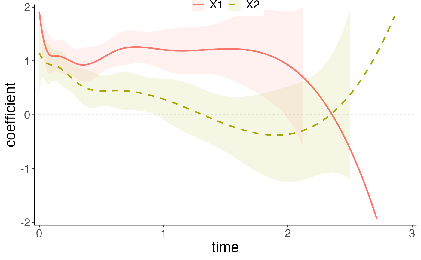
Each sub figure corresponds to a variable. It shows the time-varying effect of our predictors. In our ExampleData, the first predictor has a constant effect of 1, and the second predictor has a time-varying effect of \(\text{sin}(3\pi * t/4)\), where \(t\) is the time. The dotted line indicates the that hazard ratio is 0, which means the predictor has no effect. Users may also wish to plot the effect of different covariates in the same plot: this can be done by setting allinone = TRUE in the plot command.

The confidence interval shown presented on the figure can be calculated using the confint function.

ci.df <- confint(fit.tv)

Note that users can draw the plots by yourself with the necessary data given. We give some raw example ggplot codes. Please refer to plotting for more information.

Next we fit the Newton’s method combined with penalization method. We specify a range of penalization coefficients first, then call the coxtp function. Detailed disucussion of how to specify the range of penalization coefficients and how to choose the appropriate one will be discussed in section Information Criteria.

lambda_all <- c(1)
fit.penalize = coxtp(z = z, event = event, time=time, lambda = lambda_all, method = "ProxN")
#> Iter 1: Obj fun = -3.3017443; Stopping crit = 1.0000000e+00;
#> Iter 2: Obj fun = -3.2954100; Stopping crit = 2.0664261e-02;
#> Iter 3: Obj fun = -3.2953323; Stopping crit = 2.5346890e-04;
#> Iter 4: Obj fun = -3.2953321; Stopping crit = 4.6097119e-07;
#> Algorithm converged after 4 iterations!
#> lambda 1 is done.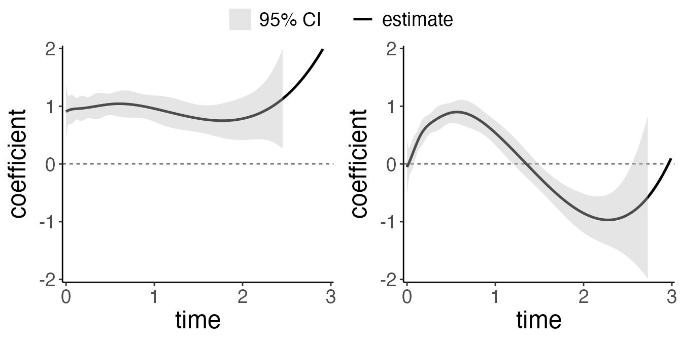

plot(fit.penalize$lambda1, ylim = c(-2,2))

With the tools introduced so far, users are able to fit the time-varying model. There are many more arguments in the package that give users a great deal of flexibility. To learn more, move on to later section.

Structure

This section gives the flowchart for the surtvep package. Generally, coxtv utilizes proximal Newton’s method to estimate the time-varying coefficients. coxtp combines the Newton’s approach with penalization. IC calculates different information criteria to select the best tuning parameter in front of the penalty term. cv.coxtp uses cross-validation for tuning parameter selection.. tvef.ph, tvef.ph.time and tvef.ph.zero provides hypothesis testing for the fitted model. get.tvef retrieves the time-varying coefficients for the fitted model. confint provides confidence intervals for these coefficients. baseline offers the baseline estimations. plot visualizes the estimated time-varying coefficients. Other functions and details are provided in later sections. Ï 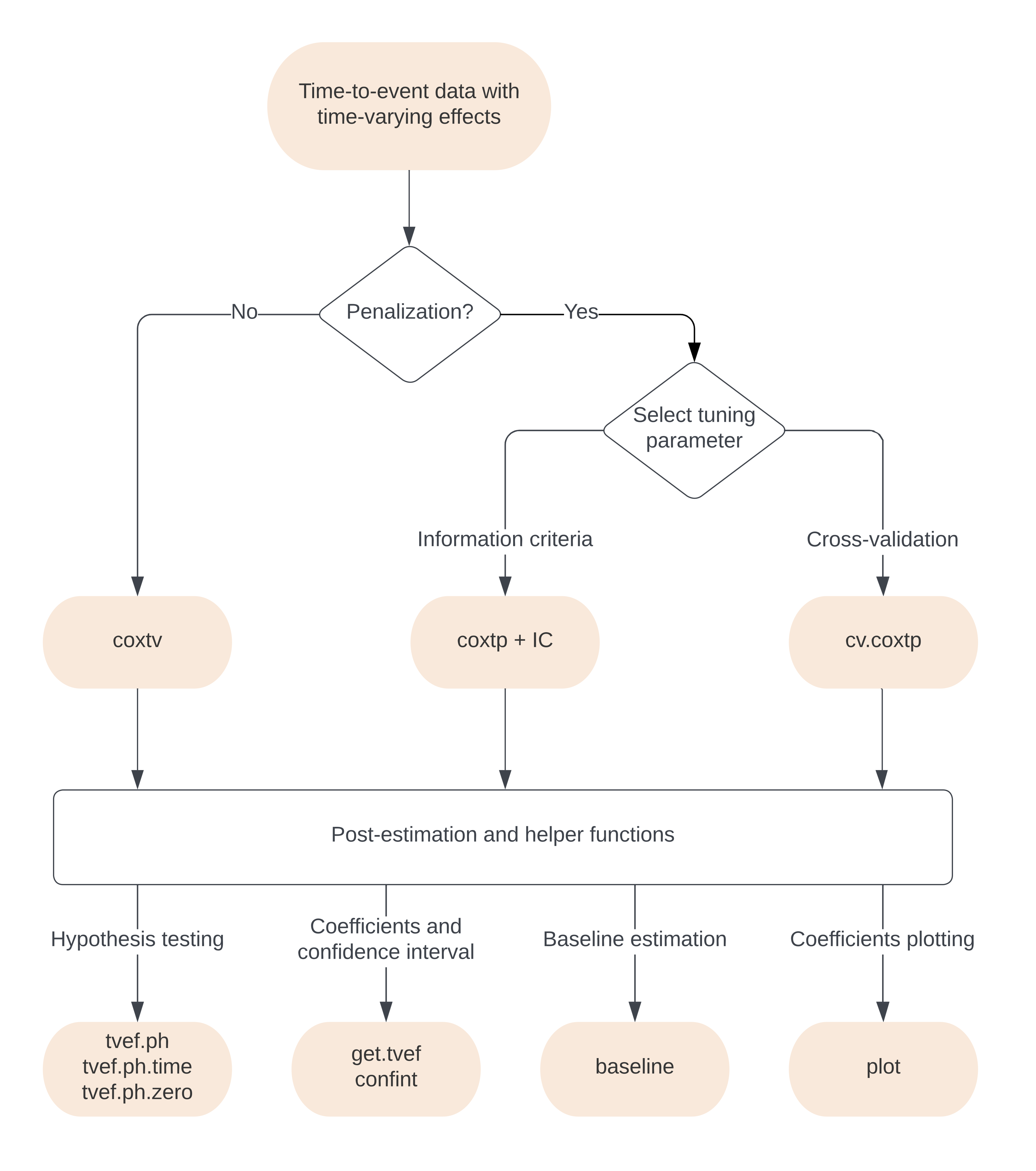Flowchart

Cox non-proportional hazards model

While obtaining these estimates under the Cox proportional-hazards model is relatively straightforward, the assumption of constant hazard ratios is frequently violated in populations defined by an initial, acute event, such as myocardial infarction, or in studies with long-term follow-up.

The Cox non-proportional hazards model is a flexible and powerful tool for modeling the time-varying effects of covariates in survival analysis, allowing for the estimation of hazard ratios that change over time. This model can capture complex relationships between predictor variables and the time-to-event outcome, providing a more accurate representation of the underlying processes.

Let \(D_{i}\) denote the time lag from transplantation to death and \(C_{i}\) be the censoring time for patient \(i\), \(i=1,\ldots, n\). Here \(n_j\) is the sample size. The observed time is \(T_{i} = \min\{D_{i},C_{i}\}\), and the death indicator is given by \(\delta_{i} = I(D_{i} \leq C_{i})\). Let \(\boldsymbol{X}_{i}=(X_{i1}, \ldots, X_{iP})^T\) be a \(P\)-dimensional covariate vector. We assume that \(D_{i}\) is independent from \(C_{i}\) given \(\textbf{X}_{i}\). Consider the hazard function \[ \lambda(t|\boldsymbol{X}_{i}) = \lambda_{0}(t)\exp\{\boldsymbol{X}_{i}^\top{\boldsymbol\beta}(t)\}, %\nonumber \] where \(\lambda_{0}(t)\) is the baseline hazard. The time-varying coefficients \(\beta(t)\) represent the effect of predictors on the outcome are varying through different time points.

To estimate the time-varying coefficients \({\boldsymbol\beta}(t)=\{\beta_{1}(t),\ldots, \beta_{P}(t)\}\), we span \(\boldsymbol\beta(\cdot)\) by a set of cubic B-splines defined on a given number of knots: \[\begin{eqnarray} \beta_{p}(t)=\boldsymbol\theta_{p}^\top\boldsymbol{B}(t)=\sum_{k=1}^K \theta_{pk} B_k(t), ~~ p=1, \ldots, P, \nonumber \end{eqnarray}\] where \(\boldsymbol{B} (t)=\{B_1(t), \ldots, B_K(t)\}^T\) forms a basis, \(K\) is the number of basis functions, and \(\boldsymbol\theta_{p}=(\theta_{p1}, \ldots, \theta_{pK})^T\) is a vector of coefficients with \(\theta_{pk}\) being the coefficient for the \(k\)-th basis of the \(p\)-th covariate. Detailed inforamtion about the construction of the B-spline basis can seen in the B-spline construction.

Newton’s method

In this section we introduce the Newton’s method for estimating time-varying effects in detail.

With a length-\(PK\) parameter vector \(\boldsymbol\theta=vec(\boldsymbol\Theta)\), the vectorization of the coefficient matrix \(\boldsymbol\Theta=(\boldsymbol\theta_{1}, \ldots, \boldsymbol\theta_{P})^T\) by row, the log-partial likelihood function is \[\begin{equation} \ell(\boldsymbol\theta)=\sum_{i=1}^{n_j} \delta_{i} \left [\boldsymbol{X}_{i}^T \boldsymbol\Theta \boldsymbol{B}(T_{i}) -\log \left\{\sum_{i' \in R_{i}} \exp \{\boldsymbol{X}_{i' }^T \boldsymbol\Theta \boldsymbol{B}(T_{i}) \} \right \} \right ] \end{equation}\], where \(R_{i}=\{i': 1 \leq i' \leq n, ~ T_{i'}\geq T_{i}\}\) is the at-risk set.

coxtv applies Newton’s method to solve the problem. Specifically, suppose we have current estimates \(\widetilde{\boldsymbol\theta}\), the update is \[ \widetilde{\boldsymbol\theta} \leftarrow \widetilde{\boldsymbol\theta} + \nu \boldsymbol{\mu}; \] where \[ \boldsymbol{\mu} = \left(- \nabla^2 \ell(\boldsymbol{\theta}) \right)^{-1} \nabla \ell(\boldsymbol{\theta}) \], and \(\nu\) is a step size adjusted by backtracking linesearch. \(\nabla \ell(\boldsymbol{\theta})\) and \(\nabla^2 \ell(\boldsymbol{\theta})\) is the first and second derivative of the log partial likelihood.

Commonly used function arguments

coxtv provides various arguments for users to customize the fit: we introduce some commonly used arguments here.

strata is a vector of indicators for stratification. Default = NULL, (i.e. no stratification group in the data), an unstratified model is implemented.
nsplines number of basis functions in the splines to span the time-varying effects, whose default value is 8. We use the R function splines::bs to generate the B-splines.
ties a character string specifying the method for tie handling. If there are no tied events, the methods are equivalent. By default "Breslow" uses the Breslow approximation, which can be faster when many ties are present.
tol tolerance used for stopping the algorithm. See details in stop below. The default value is 1e-6.
iter.max maximum iteration number if the stopping criterion specified by stop is not satisfied. Default value is 20.
degree degree of the piecewise polynomial for generating the B-spline basis functions—default is 3 for cubic splines. degree = 2 results in the quadratic B-spline basis functions.
method a character string specifying whether to use Newton method or proximal Newton method. If "Newton" then Hessian is used, while the default method "ProxN" implements the proximal Newton which can be faster and more stable when there exists ill-conditioned second-order information of the log-partial likelihood.
gammma parameter for proximal Newton method "ProxN". Default value is 1e8.
btr a character string specifying the backtracking line-search approach. "dynamic" is a typical way to perform backtracking line-search. See details in Convex Optimization by Boyd and Vandenberghe (2009). "static" limits Newton’s increment and can achieve more stable results in some extreme cases, such as ill-conditioned second-order information of the log-partial likelihood, which usually occurs when some predictors are categorical with low frequency for some categories. Users should be careful with static as this may lead to under-fitting.
tau a scalar in (0,1) used to control the step size inside the backtracking line-search. The default value is 0.5.
stop character string specifying the stopping rule to determine convergence. Use to denote the log-partial likelihood at iteration step m.
"incre" means we stop the algorithm when Newton’s increment is less than the tol. "relch" means we stop the algorithm when the is less than the tol. "ratch" means we stop the algorithm when is less than the tol. "all" means we stop the algorithm when all the stopping rules "incre", "relch" and "ratch" are met. Default value is ratch.
iter.max, if achieved, overrides any stop rule for algorithm termination.
parallel if TRUE, then the parallel computation is enabled. The number of threads in use is determined by threads.
threads an integer indicating the number of threads to be used for parallel computation. Default is 2. If parallel is false, then the value of threads has no effect.
fixedstep if TRUE, the algorithm will be forced to run iter.max steps regardless of the stopping criterion specified.

In the following sections we brefily describe these useful arguments when calling coxtv.

Now we start with a relatively harsh simulated data. Here, the covariates V1 and V2 were generated as binary variables with around 90% frequency, which is a relatively harsh setting to be estimated. The related true log-hazard function for each variable is \(\beta_1(t)=1\) and \(\beta_2(t)=exp(-1.5*t)\), where t denotes time.

Let’s check the data first:

data("ExampleDataBinary")
table(ExampleDataBinary$x[,1])
#> < table of extent 0 >
table(ExampleDataBinary$x[,2])
#> < table of extent 0 >

z     <- ExampleDataBinary$z
time  <- ExampleDataBinary$time
event <- ExampleDataBinary$event

Both predictors are presented with frequency around 25%.

Proximal Newton’s method: `method = "ProxN"`

The ‘method’ parameter has two options. method="Newton" and method="ProxN". The proximal Newton’s method modified the second order derivative \(\nabla^2 \ell(\boldsymbol{\theta})\) by adding small terms \(1/\gamma\) to the the diagonal elements. The default value of \(\gamma\) is \(10^8\), which can be modified by user. If the data set have predictors with extremely low frequency, users may consider a smaller \(\gamma\).

fit.newton <- coxtv(z = z, event = event, time = time, method = 'Newton')
fit.proxN <- coxtv(z = z, event = event, time = time, method = 'ProxN')

Then we plot the fitted methods with all the curves on the same plot. No obvious change can be oberserved here. However, we do recommand using

plot(fit.newton, ylim = c(-2,2), allinone = TRUE)
plot(fit.proxN, ylim = c(-2,2), allinone = TRUE)

Stratified Newton’s Method: `strata`

When the data of patients are collected from different strata, we can extend the model to a stratified version. We use \(j=1,\ldots,J\) to denote the \(J\) different centers. Let \(D_{ij}\) denote the time to death and \(C_{ij}\) be the censoring time for patient \(i\) in center \(j\), \(i=1,\ldots, n_j\), and \(j=1, \ldots, J\). Here \(n_j\) is the sample size in center \(j\). The total number of patients is \(N=\sum_{j=1}^Jn_j\), the observed time is \(T_{ij} = \min\{D_{ij},C_{ij}\}\), and the death indicator is given by \(\delta_{ij} = I(D_{ij} \leq C_{ij})\).

Let \(\textbf{X}_{ij}=(X_{ij1}, \ldots, X_{ijP})^T\) be a \(P\)-dimensional covariate vector. We assume that \(D_{ij}\) is independent from \(C_{ij}\) given \(\textbf{X}_{ij}\). Correspondingly, the log-partial likelihood function is \[ \ell_{strata}(\boldsymbol\theta) = \sum_{j=1}^J \sum_{i=1}^{n_j} \delta_{ij} \left [\boldsymbol{X}_{ij}^T \boldsymbol\Theta \boldsymbol{B}(T_{ij}) -\log \left\{\sum_{i' \in R_{ij}} \exp \{\boldsymbol{X}_{i' j}^T \boldsymbol\Theta \boldsymbol{B}(T_{ij}) \} \right \} \right ], \] where \(R_{ij}=\{i': 1 \leq i' \leq n_j, ~ T_{i' j}\geq T_{ij}\}\) is the at-risk set for stratum \(j\).

For the case with different strata, the usage is to include the strata variable. First, we load a set of generated data with different stratums. In our simulation, we vary the baseline for different stratums by adding a small term to the baseline function. The small term is generated by uniform distribution with mean = 0 and standard deviation = 0.5.

data("StrataExample")
z     <- StrataExample$z
time  <- StrataExample$time
event <- StrataExample$event
strata <- StrataExample$strata

The strata is a vector of indicators for stratification. The stratified model can be easily fitted by calling

fit.strata <- coxtv(z = z, event = event, time=time, strata = strata)
plot(fit.strata, ylim = c(-2,2))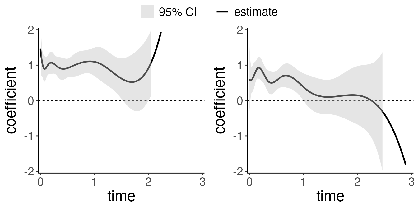

Step size adjustment: `btr`

btr is a character string specifying the backtracking line-search approach. "dynamic" is a typical way to perform backtracking line-search. See details in Convex Optimization by Boyd and Vandenberghe (2009). "static" limits Newton’s increment and can achieve more stable results in some extreme cases, such as ill-conditioned second-order information of the log-partial likelihood, which usually occurs when some predictors are categorical with low frequency for some categories.

Users should be careful with static as this may lead to under-fitting.

Newton’s Method with penalization:

The proximal Newton can help improve the estimation when the origional hessian matrix is very close to a singular one, which may often occur in the setting of time-varying effects, however, over-fitting issue still exists. We further improve the estimation by introducing the penalty. The basic idea of penalization is to control the model’s smoothness by adding a ‘wiggliness’ penalty to the fitting objective. Rather than fitting the non-proportional hazards model by maximizing original log-partial likelihood, it could be fitted by maximizing \[\begin{align} \ell(\boldsymbol{\theta}) - P_\lambda(\boldsymbol{\theta}). \end{align}\]

We have different choices of \(P_\lambda(\boldsymbol{\theta})\). Potential choices are to use P-splines, and discrete penalties. Detailed discussions are provided below.

P-spline

The P-splines are low rank smoothers using a B-spline basis, usually defined on evenly spaced knots, with a difference penalty applied directly to the parameters \(\theta_{pk}\), to control function wiggliness. When we set standard cubic B-spline basis functions, the penalty function used for \(\beta_p\) will be \[\begin{align*} P_\lambda(\boldsymbol{\theta}) = \lambda\sum_{j=1}^P\sum_{k=1}^{K-1}\{(\boldsymbol{\theta}_{j(k+1)} - \boldsymbol{\theta}_{jk})\}^2. \end{align*}\]

It is straight forward to express the penalty as a quadratic form, \(\boldsymbol{\theta}^T\boldsymbol{S}\boldsymbol{\theta}\), in this basis coefficients:

\[\begin{align*} \sum_{k=1}^{K-1}\{(\boldsymbol{\theta}_{j(k+1)} - \boldsymbol{\theta}_{jk})\}^2 = \boldsymbol{\theta}^T \begin{bmatrix} 1 & -1 & 0 & 0 & . & . & . \\ -1 & 2 & -1 & 0 & 0 & . & . \\ 0 & -1 & 2 & -1 & 0 & 0 & . \\ . & . & . & . & . & . & .\\ . & . & . & . & . & . & .\\ \end{bmatrix} \boldsymbol{\theta} \end{align*}\]

Hence the penalized fitting problem is to maximize \[\begin{align} \ell(\boldsymbol{\theta}) - \lambda\boldsymbol{\theta}^T\boldsymbol{S}\boldsymbol{\theta} \end{align}\] with respect to \(\boldsymbol{\theta}\).

Smoothing-spline

The reduced rank spline smoothers with derivative based penalties can be set up almost as easily, while retaining the sparsity of the basis and penalty and the ability to mix-and-match the orders of spline basis functions and penalties.

We denote the B-spline basis as of order \(m_1\), and \(m_1 = 3\) denotes a cubic spline. Associated with the spline will be a derivative based penalty \[\begin{align*} P_{\lambda} = \lambda \int_{0}^{T}\boldsymbol{\beta}^{[m_2]}(t)^2dt \end{align*}\] where \(\boldsymbol{\beta}^{[m_2]}(t)\) denotes the \(m_2^{th}\) derivative of \(\boldsymbol{\beta}\) with respect to \(t\). It is assumed that \(m_2 \leq m_1\), otherwise it makes no sense that the penalty is formulated in terms of a derivative that is not properly defined for the basis functions. Similarly, \(P_{\lambda}\) can be written as \(\boldsymbol{\theta}^T\boldsymbol{S}\boldsymbol{\theta}\) where \(\boldsymbol{S}\) is a banded diagonal matrix of known coefficients. The algebraic expression of \(\boldsymbol{S}\) is complex, as discussed in . However, this has little impact on the computation time.

Usage

The usage of Newton’s method with penalization coxtp is very similar to coxtv introduced above. The main difference comes from the penalization tuning parameter selection.

We use the smooth spline here for penalization (default). You could also use spline="P-spline". For tuning parameter lambda, you could either enter a single numeric value or a vector of numbers. If lambda is entered as a vector of numbers, the tuning parameter can be selected based on different criteria (AIC, TIC or GIC) using function IC. Alternatively, users can use cv.coxtp to select the tuning parameter \(\lambda\) based on cross validation.

Following is a model fit with the lambda as a vector for different illustration purposes. We use the relatively harsh setting ExampleDataBinary to illustrate the usage of coxtp, IC and cv.coxtp, the penalization method. This setting contains binary predictors with low frequency, which may have ill-conditioned second-order information of the log-partial likelihood. Penalization plays an important role here as it helps to smooth the time-varying effects.

data(ExampleDataBinary)
z     <- ExampleDataBinary$z
time  <- ExampleDataBinary$time
event <- ExampleDataBinary$event

First we fit the penalized model with "Smooth-spline".

lambda_spline_all = c(0.01,0.1,1,10,100,1000)
# fit.pspline <- coxtp(event = event, z = z, time = time, lambda=lambda_spline_all, spline = "P-spline")
fit.smoothspline <- coxtp(event = event, z = z, time = time, lambda = lambda_spline_all, penalty = "Smooth-spline")

Then we use the IC function to select the tuning parameter.

IC <- IC(fit.smoothspline)
print(IC$mAIC)
#> [1] 15209.79 15205.84 15201.74 15199.47 15199.18 15199.35
print(IC$TIC)
#> [1] 15207.09 15203.63 15199.85 15197.89 15198.62 15199.44
print(IC$GIC)
#> [1] 15208.92 15205.59 15201.99 15200.02 15199.50 15199.56

We can directly call the plot function to give the estimation plot.

plot(IC$model.TIC,ylim=c(-2,2))

From the result above, we notice that with different selection criteria, the best tuning parameter \(\lambda\) selected is different for different selection criteria. In this example, we use the TIC criterion. The result for this model is saved in the related criterion model and can be accessed as follows:

model.mAIC = IC$model.mAIC
model.TIC = IC$model.TIC
model.GIC = IC$model.GIC

Compared to the non-penalized model, we can see that the effect of ``V1” is shrunk to approximately linear in the penalized model.

Baseline estimation

The Nelson-Aalen estimator (Breslow estimator) of the cumulative function is given by \(\widetilde{\Lambda}(t) = \int_0^t \widetilde{\Lambda}_0(u)\), where \(\widetilde{\Lambda}(t)\) is 0 except at the observed failure times \(t_i\), at which it takes the value \[\begin{align*} d\Lambda_0 = {d_i}\left\{\mathop{\sum}\limits_{\ell \in R(T_i)} \exp \{\boldsymbol{X}_{i' }^T \boldsymbol{\Theta} \boldsymbol{B}(T_{i}) \}\right\}^{-1}. \end{align*}\]

The baseline estimation here refers to the baseline hazard at time t when holding all the covariates equal to zero.

data("ExampleData")
z     <- ExampleData$z
time  <- ExampleData$time
event <- ExampleData$event
time2  <- round(time, digits = 1)

lambda_spline_all=c(0.1,1,10,100)
fit.smoothspline <- coxtp(event = event, z = z, time = time2, lambda=lambda_spline_all, penalty = "Smooth-spline")
IC <- IC(fit.smoothspline)
fit.mAIC <- IC$model.mAIC

base.est = baseline(fit.mAIC)

head(base.est)
#> $time
#>  [1] 0.0 0.1 0.2 0.3 0.4 0.5 0.6 0.7 0.8 0.9 1.0 1.1 1.2 1.3 1.4 1.5 1.6 1.7 1.8
#> [20] 1.9 2.0 2.1 2.2 2.3 2.4 2.5 2.6 2.7 2.8 2.9 3.0
#> 
#> $hazard
#>  [1] 0.02576925 0.04632723 0.04796684 0.05258371 0.04708783 0.04544031
#>  [7] 0.05096521 0.03807625 0.04421912 0.05162255 0.05153851 0.06367847
#> [13] 0.04167940 0.04678650 0.04840596 0.06907205 0.05280167 0.04285638
#> [19] 0.02951995 0.02536585 0.02495845 0.02703002 0.03259201 0.03841546
#> [25] 0.01788728 0.02645356 0.02097025 0.00000000 0.03385874 0.00000000
#> [31] 0.00000000
#> 
#> $cumulHaz
#>  [1] 0.02576925 0.07209648 0.12006331 0.17264703 0.21973486 0.26517517
#>  [7] 0.31614038 0.35421663 0.39843575 0.45005830 0.50159681 0.56527528
#> [13] 0.60695468 0.65374117 0.70214714 0.77121918 0.82402086 0.86687724
#> [19] 0.89639719 0.92176304 0.94672149 0.97375150 1.00634352 1.04475898
#> [25] 1.06264625 1.08909982 1.11007006 1.11007006 1.14392881 1.14392881
#> [31] 1.14392881

As a result, we could either increase the time interval to make ties exists or remove the points that have \(\lambda=0\). The only differences would result in the baseline hazard, there is no influence on the cumulative baseline hazard.

Hypothesis Tests for the model

In this section we provide three tests for the model. The first is to test

Testing for time-varying effect

To test whether the effects are time-varying, we use the constant property of B-splines, that is, if \(\theta_{p1}=\cdots=\theta_{pK},\) the corresponding covariate effect is time-independent. Specify a matrix \(\boldsymbol{C}_p\) such that \(\boldsymbol{C}_p\boldsymbol\theta=\textbf{0}\) corresponds to the contrast that \(\theta_{p1}=\cdots=\theta_{pK}\). A Wald statistic can be constructed by \[\begin{align*} S_p=(\boldsymbol{C}_p\boldsymbol{\widehat\theta})^T \left[\boldsymbol{C}_p \{- \triangledown^2 \ell(\boldsymbol{\widehat\theta})\}^{-1}\boldsymbol{C}_p^T\right]^{-1}(\boldsymbol{C}_p\boldsymbol{\widehat\theta}). \end{align*}\]

Under the null hypothesis that the effect is time-independent, \(S_p\) is asymptotically chi-square distributed with \(K-1\) degrees of freedom.

tvef.ph(fit.proxN)
#>        chisq df          p
#> X1  6.889955  7 0.44042707
#> X2 21.437089  7 0.00317433

For the second variable, We reject the null hypothesis and claim it has the time varying effect.

Testing for beta effect

To test whether the effects are significant or not, we use the test statistic \(\theta_{p1}=\cdots=\theta_{pK} = 0,\) the corresponding covariate effect is time-independent. Specify a matrix \(\boldsymbol{C}_p\) such that \(\boldsymbol{C}_p\boldsymbol\theta=\textbf{0}\) corresponds to the contrast that \(\theta_{p1}=\cdots=\theta_{pK} = 0\). A Wald statistic can be constructed by \[\begin{align*} S_p=(\boldsymbol{C}_p\boldsymbol{\widehat\theta})^T \left[\boldsymbol{C}_p \{- \triangledown^2 \ell(\boldsymbol{\widehat\theta})\}^{-1}\boldsymbol{C}_p^T\right]^{-1}(\boldsymbol{C}_p\boldsymbol{\widehat\theta}). \end{align*}\]

test.zero <- tvef.zero(fit.proxN)

Under the null hypothesis that the effect is time-independent, \(S_p\) is asymptotically chi-square distributed with \(K\) degrees of freedom.

Testing at each time point

test.zero.time <- tvef.zero.time(fit.proxN)

From the plot above, we could observe that with different knots selected, the performance is not different so much for different knots, all the estimates are relatively close to the real function. However, in the penalized model, the lambda is more important which is another reason that we need to select the best lambda before actually fitting the model. The following plot is the performance of different lambda selected. For the following plot, the knot was set as default, which is knot=8.

Real Data Example `SUPPORT`

In this section, we illustrate the usage of our package by analyzing the time-varying effects on the real data SUPPORT (Study to Understand Prognoses Preferences Outcomes and Risks of Treatment). We use the processed SUPPORT data set included in the R package (Bhatnagar et al. 2020).

We study the time-varying effects of metastatic cancer as the illustration example and include

First we load the data and get the survival outcome:

data(support)

time <- support$d.time
death <- support$death

Age, cancer status and diabetes status are included as covariates and considered as categorical variables. Age has 4 levels, cancer status has 3 levels and diabetes has 2 levels. The following codes processed the covariates for model fitting.

#diabetes:
diabetes <-  model.matrix(~factor(support$diabetes))[,-1]

#sex: female as the reference group
sex <- model.matrix(~support$sex)[,-1]

#age: continuous variable
age <-support$age
age[support$age<=50] <- "<50"
age[support$age>50 & support$age<=60] <- "50-59"
age[support$age>60 & support$age<70] <- "60-69"
age[support$age>=70] <- "70+"
age <- factor(age, levels = c("60-69", "<50", "50-59", "70+"))
z_age <- model.matrix(~age)[,-1]

# cancer status: metastatic, yes, no
ca <- factor(support$ca)
z_ca_mets <- as.numeric(support$ca == "metastatic")
z_ca_non_mets <- as.numeric(support$ca == "yes")

z <- data.frame(z_age, z_ca_mets, z_ca_non_mets, sex, diabetes)
# colnames(z) <- c("age_50", "age_50_59", "age_70", "metastatic", "diabetes", "male")
colnames(z) <- c("age_50", "age_50_59", "age_70", "metastatic", "non_metastatic", "diabetes", "male")

The Kaplan-Meier (KM) plots were generated using the following codes to visualize the survival probability over time for three categorical variables. Analysis of the KM plot for cancer status revealed a crossover point at approximately day 200, where the survival probability of the non-metastatic cancer group surpassed that of the cancer group, suggesting a violation of the non-proportional hazards assumption.

library(survminer)
library(survival)
data <- data.frame(time, death, z)
fit1 <- survfit(Surv(time, death) ~ metastatic + non_metastatic, data = data)
fit2 <- survfit(Surv(time, death) ~ diabetes, data = data)
fit3 <- survfit(Surv(time, death) ~ age_50 + age_50_59 + age_70, data = data)
ggsurvplot(fit1, data = data, legend.labs = c("non-cancer", "non-metastatic cancer", "metastatic cancer"))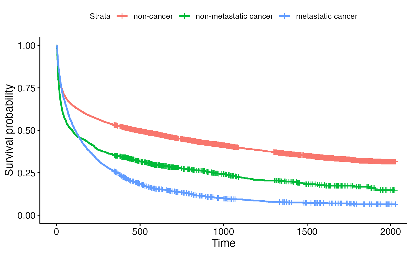

ggsurvplot(fit2, data = data, legend.labs = c("diabetes", "non-diabetes"))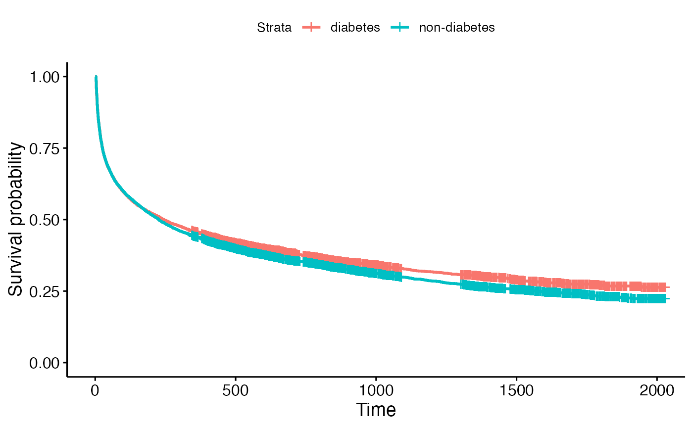

ggsurvplot(fit3, data = data, legend.labs = c("60-69", "70+", "50-59", "<50"))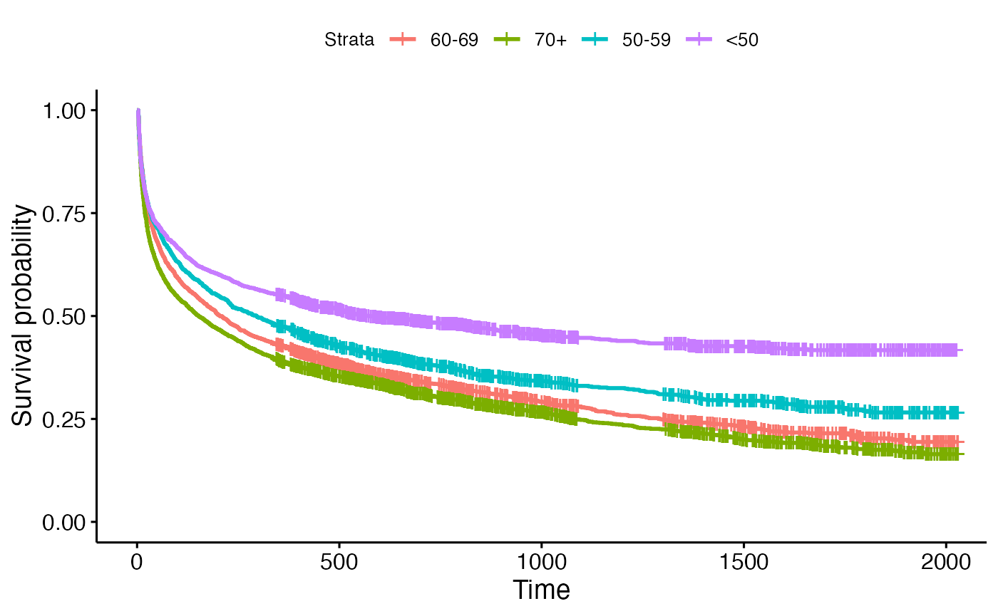

Fit the Newtons’ Method using coxtv:

fit.coxtv <- coxtv(event = death, z = z, time = time, nsplines = 10)
#> Iter 1: Obj fun = -5.7809097; Stopping crit = 1.0000000e+00;
#> Iter 2: Obj fun = -5.7668975; Stopping crit = 1.9495719e-01;
#> Iter 3: Obj fun = -5.7668366; Stopping crit = 8.4613404e-04;
#> Iter 4: Obj fun = -5.7668365; Stopping crit = 1.5189288e-06;
#> Iter 5: Obj fun = -5.7668365; Stopping crit = 1.8799714e-10;
#> Algorithm converged after 5 iterations!

We take a look at the estimation plots of cancer status using the plot function:

plot(fit.coxtv, parm = c("metastatic", "non_metastatic"), ylim = c(-2,2), ylab = "log hazard ratio")

Conditioned on the diabetes status and age, we can observe a violation of the proportional hazards assumption. A significant difference in the hazard of death was observed between the metastatic cancer, non-metastatic cancer, and non-cancer groups. Specifically, patients with metastatic cancer exhibited a higher hazard of death during the initial 1500 days compared with non-cancer patients.

However, upon examination of the estimation plot for non-metastatic cancer, a decrease at the beginning followed by an increase can be observed. The fluctuation in the plot is not deemed reliable, primarily due to the instability of the estimation. To address this issue, a penalty term was added to improve the estimation.

fit.coxtp <- coxtp(event = death, z = z, time = time, lambda = c(1,10,100,1000))
#> Iter 1: Obj fun = -5.7812444; Stopping crit = 1.0000000e+00;
#> Iter 2: Obj fun = -5.7671833; Stopping crit = 1.9641947e-01;
#> Iter 3: Obj fun = -5.7671236; Stopping crit = 8.3225826e-04;
#> Iter 4: Obj fun = -5.7671235; Stopping crit = 1.7825937e-06;
#> Iter 5: Obj fun = -5.7671235; Stopping crit = 1.4381264e-10;
#> Algorithm converged after 5 iterations!
#> lambda 1 is done.
#> Iter 1: Obj fun = -5.7812465; Stopping crit = 1.0000000e+00;
#> Iter 2: Obj fun = -5.7671838; Stopping crit = 1.9644253e-01;
#> Iter 3: Obj fun = -5.7671242; Stopping crit = 8.3187556e-04;
#> Iter 4: Obj fun = -5.7671241; Stopping crit = 1.7283676e-06;
#> Iter 5: Obj fun = -5.7671518; Stopping crit = 3.8614177e-04;
#> Iter 6: Obj fun = -5.7671241; Stopping crit = 3.8599213e-04;
#> Iter 7: Obj fun = -5.7671241; Stopping crit = 1.9834684e-13;
#> Algorithm converged after 7 iterations!
#> lambda 10 is done.
#> Iter 1: Obj fun = -5.7812812; Stopping crit = 1.0000000e+00;
#> Iter 2: Obj fun = -5.7672135; Stopping crit = 1.9659361e-01;
#> Iter 3: Obj fun = -5.7671540; Stopping crit = 8.3082429e-04;
#> Iter 4: Obj fun = -5.7671539; Stopping crit = 1.4655789e-06;
#> Iter 5: Obj fun = -5.7673043; Stopping crit = 2.1045372e-03;
#> Iter 6: Obj fun = -5.7671539; Stopping crit = 2.1001131e-03;
#> Iter 7: Obj fun = -5.7671539; Stopping crit = 8.0611971e-13;
#> Algorithm converged after 7 iterations!
#> lambda 100 is done.
#> Iter 1: Obj fun = -5.7814771; Stopping crit = 1.0000000e+00;
#> Iter 2: Obj fun = -5.7674171; Stopping crit = 1.9704674e-01;
#> Iter 3: Obj fun = -5.7673576; Stopping crit = 8.3362394e-04;
#> Iter 4: Obj fun = -5.7673575; Stopping crit = 1.3752688e-06;
#> Iter 5: Obj fun = -5.7675286; Stopping crit = 2.4012175e-03;
#> Iter 6: Obj fun = -5.7673575; Stopping crit = 2.3954592e-03;
#> Iter 7: Obj fun = -5.7673575; Stopping crit = 1.0074129e-12;
#> Algorithm converged after 7 iterations!
#> lambda 1000 is done.
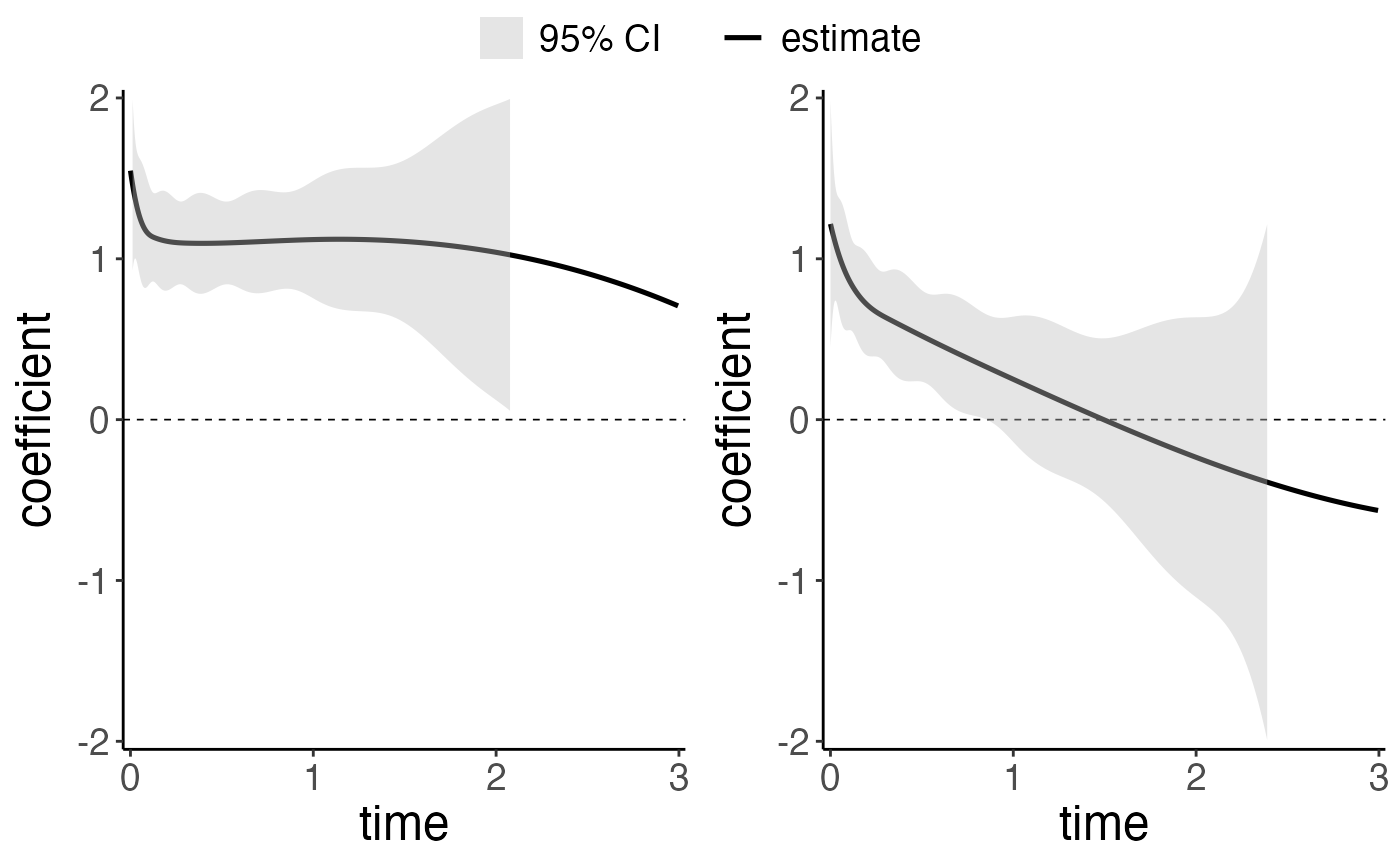
IC.support <- IC(fit.coxtp)

plot(IC.support$model.mAIC, parm = c("metastatic", "non_metastatic"), ylim = c(-2,2), ylab = "log hazard ratio")

Then we provide the hypothesis testing for each covariate.

#test the proportional hazards assumption
test.ph <- tvef.ph(fit.coxtv)
print(test.ph)
#>                     chisq df            p
#> age_50          46.311169  9 5.271760e-07
#> age_50_59       13.208472  9 1.533978e-01
#> age_70           3.338770  9 9.493378e-01
#> metastatic     389.789436  9 2.064355e-78
#> non_metastatic   4.168983  9 8.999424e-01
#> diabetes        19.018021  9 2.504010e-02
#> male            44.476142  9 1.153035e-06

#test the significance of each covariate
test.zero <- tvef.zero(fit.coxtv)
print(test.zero)
#>                    chisq df             p
#> age_50          92.95934 10  1.384020e-15
#> age_50_59       23.20617 10  1.001062e-02
#> age_70          33.59559 10  2.162004e-04
#> metastatic     997.76510 10 5.666717e-208
#> non_metastatic 134.96747 10  4.517433e-24
#> diabetes        25.96236 10  3.791138e-03
#> male            48.35095 10  5.354766e-07

When testing for the proportional hazards assumption, age_50, non_cancer, non_metastatic, diabetes and male has p-value < 0.05. We reject the null hypothesis and claim that these covariates have violated the proportional hazards assumption.

All these covariates are significant based on the Wald test.

Then we can use the following codes to get the baseline estimation and the baseline plot.

base <- baseline(IC.support$model.TIC)

plot(base)

When dealing with data where ties are presented, we can also give baseline hazard and absolute hazard for each covariate.

We utilized the Breslow’s approximation to estimate the baseline hazard at each event time. We round the unique event time first.

time.discrete <- round(support$d.time, digits = -2)

fit.discrete <- coxtv(event = death, z = z, time = time.discrete, nsplines = 10)
#> Iter 1: Obj fun = -5.8724904; Stopping crit = 1.0000000e+00;
#> Iter 2: Obj fun = -5.8627640; Stopping crit = 1.6318989e-01;
#> Iter 3: Obj fun = -5.8627181; Stopping crit = 7.6917032e-04;
#> Iter 4: Obj fun = -5.8627180; Stopping crit = 1.5741850e-06;
#> Iter 5: Obj fun = -5.8627180; Stopping crit = 1.9209980e-10;
#> Algorithm converged after 5 iterations!

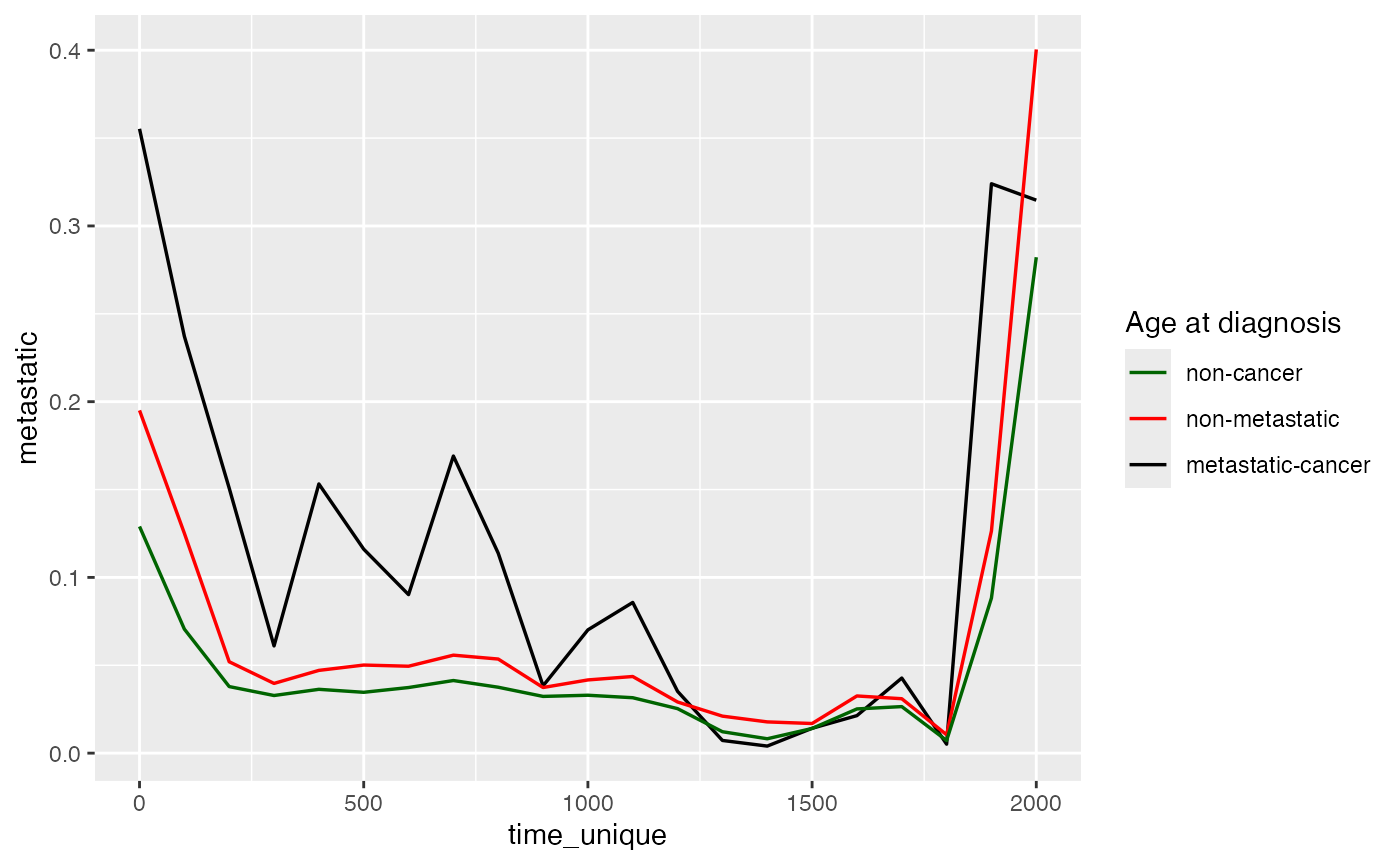
base.discrete <- baseline(fit.discrete)

The following codes provide the absolute hazards plot.

beta.abso <- data.frame(get.tvcoef(fit.discrete))

time_unique<- unique(time.discrete)

haz_j      <- base.discrete$hazard

smooth_data <- data.frame(time_unique, haz_j)

loessMod30 <- loess(haz_j ~ time_unique, data=smooth_data, span=0.30) # 30% smoothing

haz_j_smooth30 <- predict(loessMod30)

exp_betax<- matrix(0,length(unique(time.discrete)),dim(z)[2])
beta2                   <- beta.abso
beta2$cancer         <- 0

exp_betax               <- exp(beta2)

haz_0_betax             <- haz_j_smooth30 * exp_betax

library(ggplot2)
plot_age <- ggplot(haz_0_betax, aes(x=time_unique)) +
  geom_line(aes(y=metastatic,  color = "metastatic-cancer"),size = 0.6) +
  geom_line(aes(y=non_metastatic,    color = "non-metastatic"),size = 0.6) +
  geom_line(aes(y=cancer,  color = "non-cancer"),size = 0.6) +
  scale_color_manual(name='Age at diagnosis',
                     breaks = c('non-cancer', 'non-metastatic', 'metastatic-cancer'),
                     values = c('non-cancer'='dark green', 'non-metastatic'='red', 'metastatic-cancer' = 'black')) +
  theme(plot.title = element_text(hjust = 0.2))
#> Warning: Using `size` aesthetic for lines was deprecated in ggplot2 3.4.0.
#> ℹ Please use `linewidth` instead.
#> This warning is displayed once every 8 hours.
#> Call `lifecycle::last_lifecycle_warnings()` to see where this warning was
#> generated.
plot_age

Bhatnagar, Sahir, Maxime Turgeon, Jesse Islam, Olli Saarela, and James Hanley. 2020. “Casebase: Fitting Flexible Smooth-in-Time Hazards and Risk Functions via Logistic and Multinomial Regression.” https://CRAN.R-project.org/package=casebase.