survkl: Transfer-Learning Based Integrated Cox Models

Introduction

Accurate prognosis prediction plays a central role in survival analysis. The recent growth of large-scale biobank studies—characterized by extensive genetic, transcriptomic, imaging, and electronic health record data—has created new opportunities to enhance prediction accuracy. However, despite their potential, these datasets often suffer from limited effective sample sizes, high dimensionality, low signal-to-noise ratios, and practical constraints such as patient privacy.

Integrating external information is a promising strategy for improving model performance, yet classical data integration methods typically assume homogeneous data-generating mechanisms across sources. This assumption rarely holds in modern biomedical applications. Ignoring heterogeneity can introduce substantial bias, underscoring the need for transfer-learning approaches that explicitly account for discrepancies across populations.

While KL divergence has been used previously for integrating binary-outcome models, extending such ideas to censored time-to-event outcomes is nontrivial due to censoring and the limited nature of available external survival information (e.g., predicted risk scores or sets of coefficients without a baseline hazard).

The survkl package addresses these challenges by offering a transfer-learning framework for Cox models that integrates external information with newly collected survival data. It is designed to be flexible, privacy-preserving, and effective across both low- and high-dimensional settings. Key features include:

Key Features

• Transfer Learning with KL Integration:
  Incorporates various types of external information via KL-based penalization to adaptively borrow strength.

• Privacy-Preserving External Use:
  Requires only summary-level external inputs—such as risk scores or coefficient estimates—without access to individual-level external data.

• Robustness to Heterogeneity:
  Explicitly accounts for population differences through adaptive weighting controlled by tuning parameters (eta), enabling selective borrowing from compatible sources.

• High-Dimensional Modeling Support:
  Implements regularized KL-integrated Cox models, including

  • Ridge (coxkl_ridge)
    
  • Elastic Net (coxkl_enet, including LASSO as a special case)

• Flexible External Information Formats:
  Supports external coefficients, risk scores, and partially overlapping predictor sets.

• Comprehensive Cross-Validation Framework:
  Provides multiple tuning criteria including

  • Two based on C-index
    
  • Two based on Loss: predicted deviance and V&VH loss.

This vignette introduces the main functionalities of survkl and provides examples for both low- and high-dimensional modeling workflows.

Installation

You can install from CRAN:

install.packages("survkl")

Or install the development version of survkl from GitHub:

require(devtools)
require(remotes)
remotes::install_github("UM-KevinHe/survkl", ref = "main")

Quick Start

This section provides a brief overview of the main functions using example datasets included in the package.

First, load the package:

library(survkl)

Low-Dimensional Integration

The low-dimensional KL-integrated Cox model, implemented in coxkl, is designed for settings where the number of predictors is modest. The method incorporates external information—either in the form of external Cox coefficients (beta) or pre-computed external risk scores (RS)—using a KL-based penalization. The tuning parameter eta governs the degree of borrowing:
- eta = 0 reproduces the standard Cox model;
- larger eta values increasingly pull the fitted coefficients toward the external information.

In this section we demonstrate how to fit a KL-integrated Cox model and how to select the optimal eta using cross-validation via cv.coxkl.

Example data structure

We illustrate the workflow using the built-in low-dimensional simulated dataset:

data(ExampleData_lowdim)

train  <- ExampleData_lowdim$train
test   <- ExampleData_lowdim$test

z      <- train$z
delta  <- train$status
time   <- train$time
strat  <- train$stratum

and externally derived coefficients beta_external:

beta_ext <- ExampleData_lowdim$beta_external_good

We generate a sequence of eta values through the internal utility generate_eta(), and fit the KL-integrated model across this grid:

eta_grid <- generate_eta(method = "exponential", n = 100, max_eta = 30)
fit_lowdim <- coxkl(
  z = z,
  delta = delta,
  time = time,
  stratum = strat,
  beta = beta_ext,
  etas = eta_grid
)

The S3 method coef() provides a clean interface to extract estimated coefficients. If the requested eta is between fitted values, linear interpolation is performed:

coef(fit_lowdim, eta = 1)

## Warning: Linear interpolation performed between eta = 0.979 and eta = 1.040 for
## eta = 1.000.

##                1
## [1,]  0.25018459
## [2,] -0.39555046
## [3,]  0.08825084
## [4,] -0.58446411
## [5,]  0.29503025
## [6,] -0.55443656

Users may instead supply an external risk score vector:

RS_ext <- as.matrix(z) %*% as.matrix(beta_ext)

fit_lowdim_RS <- coxkl(
  z = z,
  delta = delta,
  time = time,
  stratum = strat,
  RS = RS_ext,
  etas = eta_grid
)

coef(fit_lowdim_RS)[1:5]

## [1]  0.25982263 -0.49599768 -0.01972113 -0.84023506  0.24808718

Objects of class coxkl can be visualized using the S3 plotting method plot().
This function displays how model performance changes across the eta–sequence used during fitting.

Two types of performance criteria are supported:

• "loss"
  (default; −2 × partial log-likelihood, normalized by sample size)

• "CIndex"
  (stratified concordance index)

If no test data are supplied, performance is computed using the training data stored in object$data:

plot(
  fit_lowdim,
  test_z       = test$z,
  test_time    = test$time,
  test_delta   = test$status,
  test_stratum = test$stratum,
  criteria     = "loss"
)    

## Warning: Using `size` aesthetic for lines was deprecated in ggplot2 3.4.0.
## ℹ Please use `linewidth` instead.
## ℹ The deprecated feature was likely used in the survkl package.
##   Please report the issue to the authors.
## This warning is displayed once every 8 hours.
## Call `lifecycle::last_lifecycle_warnings()` to see where this warning was
## generated.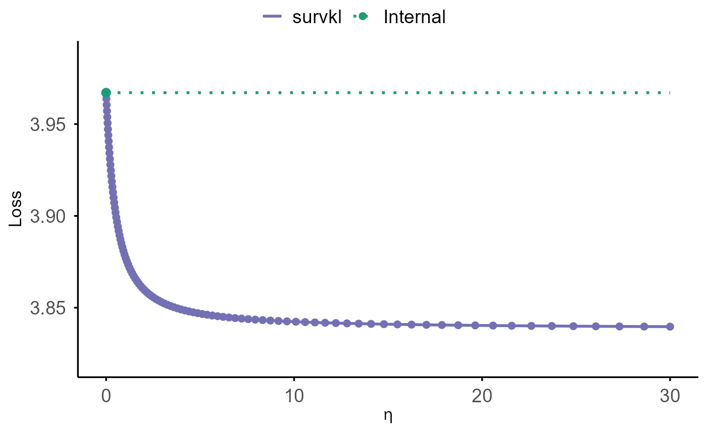

The function cv.coxkl performs K-fold (default 5) cross-validation to choose the integration parameter. It supports four criteria:

• "V&VH" — V&VH loss
  
• "LinPred" — predicted partial deviance
  
• "CIndex_pooled" — pooled comparable pairs
  
• "CIndex_foldaverage" — per-fold stratified C-index

Below is an example using the default "V&VH" criterion:

cv_lowdim <- cv.coxkl(
  z        = z,
  delta    = delta,
  time     = time,
  stratum  = strat,
  beta     = beta_ext,
  etas     = eta_grid,
  nfolds   = 5,
  criteria = "V&VH",
  seed = 1)

The cross-validated performance curve can be visualized using cv.plot():

cv.plot(cv_lowdim)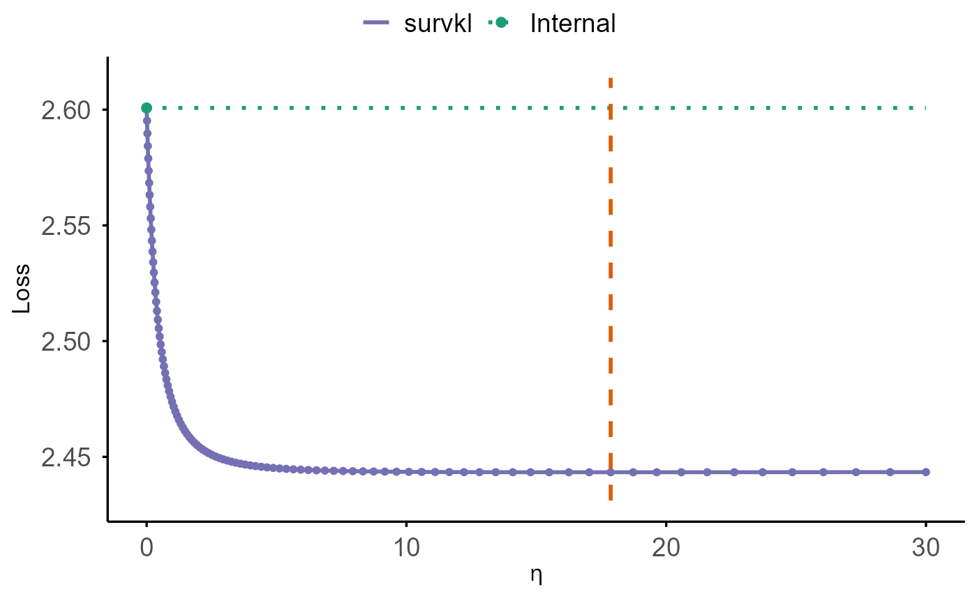

The solid purple curve displays the cross-validated loss across different values of eta. The green dotted horizontal line marks the internal baseline at eta = 0, representing the model that does not incorporate external information. The vertical dashed orange line indicates the optimal eta value, where the cross-validated loss is minimized.

A comparison between the purple curve and the green baseline shows whether borrowing external information improves prediction performance. Whenever the purple curve falls below the green line, using external information (eta > 0) yields better predictive accuracy than relying solely on the internal model.

High-Dimensional Integration (Ridge, Elastic Net, and LASSO)

In high-dimensional settings (for example, when the number of predictors is comparable to or exceeds the sample size), the survkl package extends KL-integrated Cox modeling with regularization. Two families of penalties are supported:

• Ridge penalty (L2), implemented in coxkl_ridge, which shrinks all coefficients toward zero while retaining dense solutions.
• Elastic net penalty (a mixture of L1 and L2), implemented in coxkl_enet, which includes the LASSO (pure L1) as a special case when the mixing parameter is set to 1.

Both models combine:

• a KL term, controlled by the integration parameter eta, to borrow information from external sources (risk scores RS or coefficients beta), and
  
• a regularization term (ridge or elastic net) to stabilize estimation in high-dimensional designs.

In this section we first introduce the shared high-dimensional example dataset, and then illustrate the usage of the ridge-penalized model coxkl_ridge. (The elastic net workflows are analogous and will be discussed in a separate subsection.)

High-dimensional example data

We use the built-in high-dimensional simulated dataset:

data(ExampleData_highdim)

train_hd  <- ExampleData_highdim$train
test_hd   <- ExampleData_highdim$test

z_hd      <- train_hd$z
delta_hd  <- train_hd$status
time_hd   <- train_hd$time
strat_hd  <- train_hd$stratum

This dataset contains 50 predictors (Z1–Z50) with 6 signal variables and 44 AR(1) noise variables. Externally derived coefficients are provided in beta_external:

beta_external_hd <- ExampleData_highdim$beta_external

These external coefficients are estimated from a separate dataset using only Z1–Z6 and then expanded to a length-50 vector, with zeros for Z7–Z50.

Ridge-Penalized KL-Integrated Cox Model (coxkl_ridge)

The function coxkl_ridge fits a KL-integrated Cox model with a ridge (L2) penalty on all predictors. External information is incorporated through a KL term weighted by eta (an user-specified scalar), while the ridge penalty is controlled by a sequence of tuning parameters lambda. If lambda is not provided, a decreasing lambda path is generated automatically.

We first fit a KL–ridge model for a fixed integration weight eta and an automatically generated lambda path:

model_ridge <- coxkl_ridge(
  z        = z_hd,
  delta    = delta_hd,
  time     = time_hd,
  stratum  = strat_hd,
  beta     = beta_external_hd,   # external coefficients (length 50)
  eta      = 1                  # KL integration weight
)

The fitted object stores, for each lambda value:

• model_ridge$lambda — the lambda sequence (in decreasing order),
• model_ridge$beta — estimated coefficients (one column per lambda),
• model_ridge$linear.predictors — linear predictors for all observations and all lambda values,
• model_ridge$likelihood — partial log-likelihood along the lambda path,
• model_ridge$data — the data used for fitting.

The S3 method coef() extracts the estimated coefficients:

# All lambdas (columns ordered in decreasing lambda)
coef(model_ridge)[1:5, 1:5]  # first 5 lambdas

##          82.0989     74.8055     68.1599     62.1048     56.5876
## [1,]  0.03940019  0.04317345  0.04718185  0.05142086  0.05588316
## [2,] -0.08703965 -0.09270340 -0.09863286 -0.10483116 -0.11129985
## [3,]  0.04654658  0.05031996  0.05434817  0.05864173  0.06321089
## [4,] -0.05680339 -0.06147303 -0.06646655 -0.07179722 -0.07747730
## [5,]  0.10912724  0.11518227  0.12137484  0.12769148  0.13411779

To focus on a specific value of lambda:

lambda_target <- model_ridge$lambda[5]
coef(model_ridge, lambda = lambda_target)[1:5]

## [1]  0.05588316 -0.11129985  0.06321089 -0.07747730  0.13411779

If the requested lambda is not exactly one of the fitted values, coef() performs linear interpolation along the lambda path.

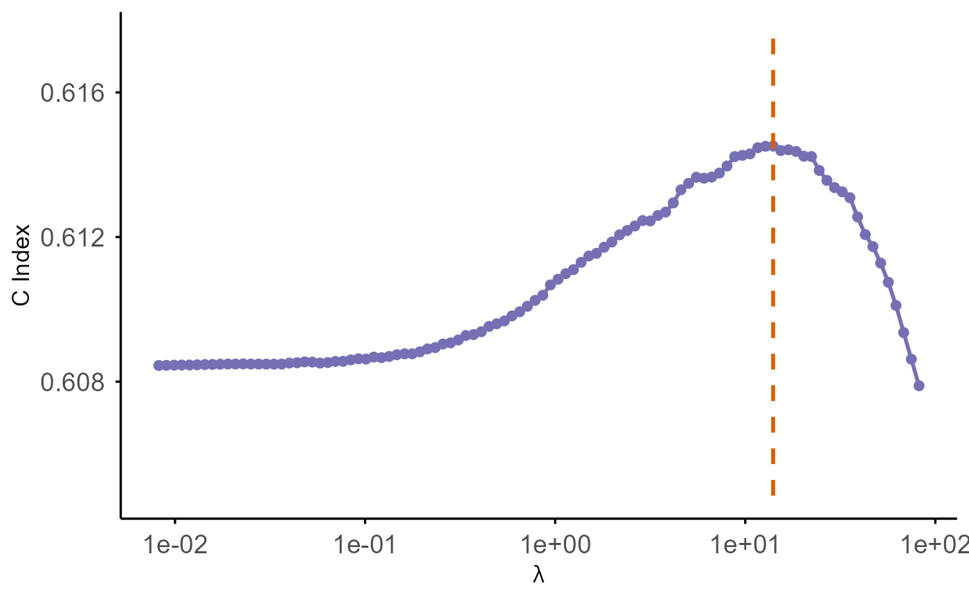
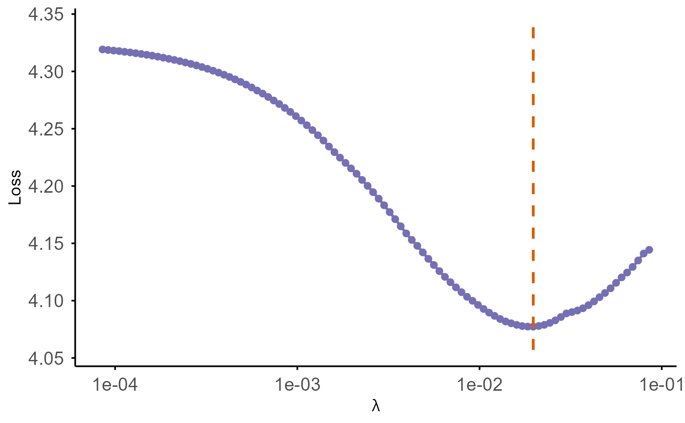
Objects of class coxkl_ridge can be visualized using the S3 plotting method plot():

By default, this plots (at given eta):

• Loss (-2 * partial log-likelihood) versus the penalty parameter lambda,
• x-axis on a reversed log10 scale (larger penalties on the left, smaller penalties on the right),
• y-axis labeled as “Loss”.
• A vertical dashed orange line marks the optimal value of λ, where the loss reaches its minimum on the evaluated grid.

plot(
  model_ridge,
  test_z       = test_hd$z,
  test_time    = test_hd$time,
  test_delta   = test_hd$status,
  test_stratum = test_hd$stratum,
  criteria     = "CIndex"
)

The function cv.coxkl_ridge performs K-fold cross-validation to tune the integration parameter eta while internally scanning over a lambda path for each candidate eta. For each eta, it:

• evaluates a sequence of ridge penalties lambda,
• computes the chosen cross-validation criterion on held-out folds,
• selects the best lambda for that eta,
• aggregates the results into summary tables.

Supported criteria are:

• "V&VH" — V&VH loss (reported as Loss = -2 * score),
• "LinPred" — predicted partial deviance,
• "CIndex_pooled" — pooled C-index over all folds,
• "CIndex_foldaverage" — average C-index across folds.

Example: tuning eta using 5-fold cross-validation and the "V&VH" criterion:

eta_grid_hd <- generate_eta(method = "exponential", n = 50, max_eta = 100)

cv_ridge_hd <- cv.coxkl_ridge(
  z           = z_hd,
  delta       = delta_hd,
  time        = time_hd,
  stratum     = strat_hd,
  beta        = beta_external_hd,
  etas        = eta_grid_hd,
  nfolds      = 5,
  cv.criteria = "V&VH",
  seed = 1)

The best lambda for each eta (according to the chosen criterion) is provided by:

cv_ridge_hd$integrated_stat.best_per_eta

##             eta       lambda     Loss
## 1    0.00000000 1.025724e+02 2.821608
## 2    0.09953651 9.834014e+01 2.818411
## 3    0.20888146 9.449421e+01 2.815652
## 4    0.32900138 7.554877e+01 2.813131
## 5    0.46095806 5.515441e+01 2.810267
## 6    0.60591790 4.034998e+01 2.806921
## 7    0.76516225 2.957942e+01 2.803008
## 8    0.94009872 2.029238e+01 2.798498
## 9    1.13227362 1.545093e+01 2.793370
## 10   1.34338567 1.071272e+01 2.787729
## 11   1.57530093 7.423356e+00 2.781748
## 12   1.83006939 5.642671e+00 2.775576
## 13   2.10994303 3.906313e+00 2.769394
## 14   2.41739573 2.703155e+00 2.763368
## 15   2.75514517 1.869880e+00 2.757622
## 16   3.12617683 1.293037e+00 2.752276
## 17   3.53377037 7.421110e-01 2.747417
## 18   3.98152865 3.879752e-01 2.743117
## 19   4.47340953 1.057312e-01 2.739418
## 20   5.01376093 8.595137e-03 2.736400
## 21   5.60735916 8.612383e-03 2.734238
## 22   6.25945124 8.628077e-03 2.732777
## 23   6.97580122 8.642360e-03 2.731864
## 24   7.76274115 8.655359e-03 2.731377
## 25   8.62722703 8.667188e-03 2.731219
## 26   9.57690034 8.677955e-03 2.731312
## 27  10.62015555 8.687754e-03 2.731591
## 28  11.76621431 8.696673e-03 2.732009
## 29  13.02520701 8.704790e-03 2.732525
## 30  14.40826229 8.712178e-03 2.733107
## 31  15.92760542 8.718903e-03 2.733730
## 32  17.59666636 8.725024e-03 2.734376
## 33  19.43019846 8.730595e-03 2.735029
## 34  21.44440891 8.735666e-03 2.735677
## 35  23.65710197 8.740282e-03 2.736313
## 36  26.08783632 8.744483e-03 2.736929
## 37  28.75809801 8.748307e-03 2.737521
## 38  31.69149033 8.751788e-03 2.738086
## 39  34.91394249 8.754956e-03 2.738622
## 40  38.45393876 8.757841e-03 2.739128
## 41  42.34277030 8.760466e-03 2.739603
## 42  46.61481175 8.762856e-03 2.740048
## 43  51.30782504 8.765031e-03 2.740464
## 44  56.46329322 8.767011e-03 2.740851
## 45  62.12678712 8.768813e-03 2.741211
## 46  68.34836818 8.770454e-03 2.741544
## 47  75.18303094 8.771947e-03 2.741852
## 48  82.69118918 8.773307e-03 2.742137
## 49  90.93920990 8.774544e-03 2.742399
## 50 100.00000000 8.775671e-03 2.742641

As with low-dimensional models, the helper function cv.plot() can be used to visualize performance versus eta:

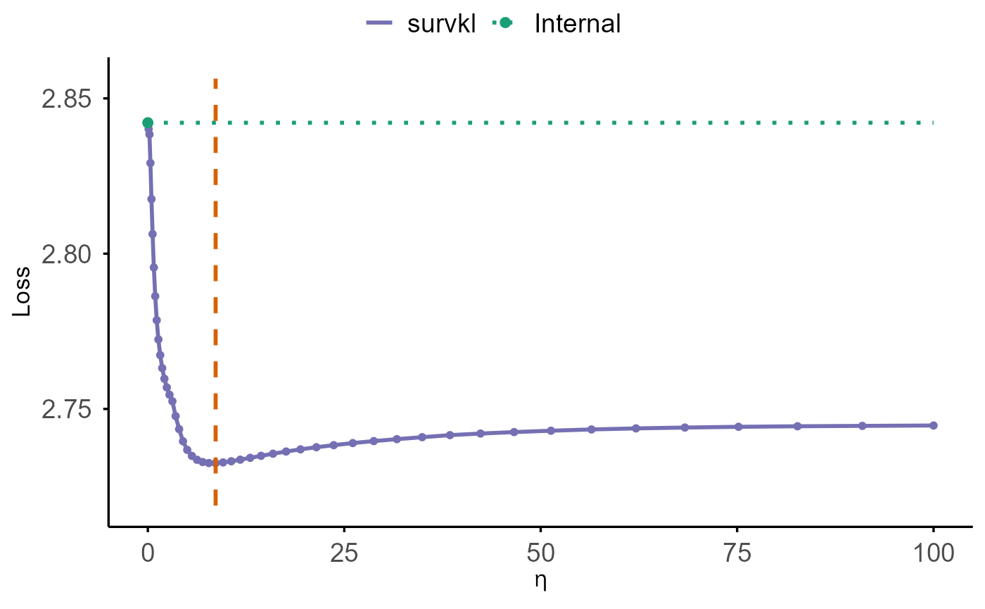
cv.plot(cv_ridge_hd)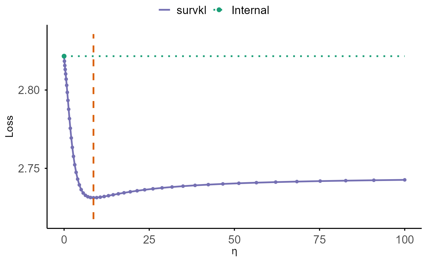

The plot shows:

• a purple curve for the cross-validated performance across the eta sequence (loss or C-index),
• a green dotted horizontal line indicating the internal baseline at eta = 0,
• a green point marking the baseline value,
• and a vertical dashed orange line indicating the optimal η, where the cross-validated loss reaches its minimum.

Elastic-Net / LASSO KL-Integrated Cox Model (coxkl_enet)

The function coxkl_enet fits a KL-integrated Cox model with an elastic-net penalty, controlled by the mixing parameter alpha. When alpha = 1, the penalty reduces to LASSO, enabling coefficient sparsity in addition to KL-based integration of external information.

External knowledge may be incorporated either through external coefficients (beta) or an externally computed risk score (RS). The integration weight eta determines how strongly the model borrows from this external signal, while the penalty parameter lambda controls the sparsity level. If lambda is not supplied, the function automatically generates a decreasing lambda sequence.

We illustrate the workflow using LASSO (alpha = 1) with an automatically generated lambda path:

model_enet <- coxkl_enet(
  z        = z_hd,
  delta    = delta_hd,
  time     = time_hd,
  stratum  = strat_hd,
  beta     = beta_external_hd,   
  eta      = 1,                 
  alpha    = 1                  # LASSO penalty
)

The fitted object stores, for each lambda value:

• model_enet$lambda — the lambda sequence (in decreasing order),
• model_enet$beta — estimated coefficients (one column per lambda),
• model_enet$likelihood — partial log-likelihood along the lambda path,
• model_enet$data — the data used for fitting.

The S3 method coef() extracts the estimated coefficients:

coef(model_enet)[1:5, 1:5]

##    0.0853     0.0796     0.0742     0.0692     0.0645
## Z1      0 0.00000000 0.00000000 0.00000000 0.00000000
## Z2      0 0.00000000 0.00000000 0.00000000 0.00000000
## Z3      0 0.00000000 0.00000000 0.00000000 0.00000000
## Z4      0 0.00000000 0.00000000 0.00000000 0.00000000
## Z5      0 0.01945713 0.03849402 0.05620049 0.07282693

To extract coefficients corresponding to a specific lambda:

lambda_target <- model_enet$lambda[5]
coef(model_enet, lambda = lambda_target)[1:5]

## [1] 0.00000000 0.00000000 0.00000000 0.00000000 0.07282693

Objects of class coxkl_enet can be visualized using the S3 method plot(), and default is to plot loss versus lambda:

plot(
  model_enet,
  test_z = test_hd$z,
  test_time = test_hd$time,
  test_delta = test_hd$status,
  test_stratum = test_hd$stratum,
  criteria = "loss"
)

Similar, the function cv.coxkl_enet extends the above fitting procedure by performing K-fold cross-validation over a supplied grid of eta values:

eta_grid_hd <- generate_eta(method = "exponential",
                            n = 50,
                            max_eta = 100)

cv_enet_hd <- cv.coxkl_enet(
  z = z_hd,
  delta = delta_hd,
  time = time_hd,
  stratum = strat_hd,
  beta = beta_external_hd,
  etas = eta_grid_hd,
  alpha = 1, # LASSO
  nfolds = 5,
  cv.criteria = "V&VH",
  seed = 1
)

CV results can be visualized using cv.plot():

cv.plot(cv_enet_hd)